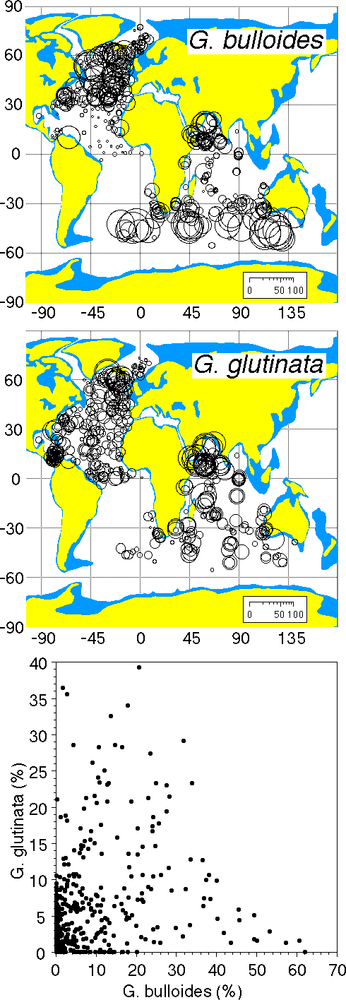
Relations of G. bulloides and G. glutinata
Only few samples exist in the CLIMAP Holocene data in which
both species do not co-occur (Fig. 40). Their relative abundances
show some inverse correlation. Globigerina bulloides is more
abundant in central upwelling zones and areas of high productivity
while G. glutinata is more frequent at their margins and in central
ocean areas. This is well expressed in the biogeographic maps
of Bé and Hutson (1977) in the area of upwelling in the
Arabian Sea offshore from Somalia. The central area is occupied
by abundant G. bulloides, while a belt with abundant G. glutinata
exists in the marginal upwelling zone (see also Brock et al.,
1992). Globigerina bulloides feeds on algal prey (Lee et al.,
1966), while G. glutinata has more specific preferences for diatoms
(Hemleben et al., 1989). Such different feeding strategies may
explain why both species are related to productive environments
but tend to occupy different zones, probably related to the phytoplankton
bloom succession (dinoflagellates - diatoms).
Relations of G. calida and G. siphonifera
It is difficult to argue about possible taxonomic uncertainties
in the counts of G. calida and G. siphonifera and subsequent
problems in the interpretation of their relations with the physical
environment. CLIMAP micropaleontologists have made serious efforts
for quality control of their micropaleontologic data and taxonomic
standardisation between the different members of the group. Other
species, which are difficult to distinguish in their morphology
(e.g. G. falconensis and G. bulloides) have distinctly different
adaptations and suggest that the similarities in the ecologic
pattern between G. calida and G. siphonifera are real. This problem
may suggest to include both species in one taxonomic category
and demands for taxonomic research.
Relations of G. rubescens and G. tenella
Globoturborotalita tenella is distinguished from the generally
pink-colored G. rubescens by a secondary aperture on the last
chamber. Pre-adult stages of G. rubescens and G. tenella are
difficult to distinguish in their morphologies and taxonomic
discrimination is made more difficult by the existence of a white
form of G. rubescens in bottom sediments of temperate regions
(Hemleben et al., 1989). Morphologic similarities and the nearly
equal relations with the physical environment seen in G. rubescens
and G. tenella may suggest ecophenotypes rather than different
species. In other species variants are consistently more differentiated
in their preferences compared to G. rubescens and G. tenella.
Both species require taxonomic and ecologic research.
Relations of G. sacculifer and S. dehiscens
Bé (1965) considered S. dehiscens as a deep-water form
of G. sacculifer in a terminal (reproductive) stage. In the laboratory,
however, Glbigerinoides sacculifer was observed during gamete
release and did not develop the "S. dehiscens" form
(Hemleben et al., 1987). Other authors emphasize morphological
differences in juvenile stages of the two species (Hemleben et
al., 1989). Pattern in the plots of relative abundances vs. physical
parameters, however, is very similar for G. sacculifer and S.
dehiscens. Both species differ drastically in their relative
abundances and comparisons of their relations with the physical
environment are difficult. The correlation coefficients of their
relative abundances computed with various regression methods
are all well below 0.1. This, however, may be caused by the low
relative abundance of S. dehiscens (< 5 %) which causes statistical
uncertainty due to counting error in the data. Potentially, S.
dehiscens may occupy a deep-water habitat with a biogeographic
distribution similar to that of G. sacculifer. The possible existence
of vertical clines in phenotypes, in contrast to the commonly
observed geographic clines in other species, motivates more research
on relations of the two species.
G. crassaformis and G. truncatulinoides
The origin of G truncatulinoides as a species, about 2.8 -
2.9 My ago, was analysed in a morphometric study by Lazarus et
al. (1995). They suggested a sympatric mode of evolution, in
which the differentiation and "geographic isolation"
of ancestor (G. crassaformis) and descendant species (G. truncatulinoides)
occurs through the occupation of different niches (e.g. depth
habitats, seasonally different cycles, etc.) in the same biogeographic
region (see discussion by Lazarus et al., 1995). The substantially
different specialisations of both species seen in the relations
with the physical environment (Figs. 19 and 24) support this
view.
Dominant species
Table 1 lists those species which dominate at least one of
the 461 samples used in this study. Only six species, however,
can be considered as dominant species on a biogeographic scale:
N. pachyderma, G. inflata, G. bulloides, G. ruber, G. glutinata,
and G. menardii. Broad relations with sea surface temperatures
in distinct biogeographic provinces exist for N. pachyderma in
the polar and subpolar provinces, G. inflata in the transitional
province, G. ruber in the subtropical and tropical province,
and G. menardii in the warm tropical province. The latter species
is not commonly a dominant species and may reflect selective
dissolution (Kipp, 1976). Globigerina bulloides and G. glutinata
dominate in productive high latitude environments and areas of
upwelling. The biogeographic relations suggest different preferences
of the two species for the central and marginal oceanographic
and biologic conditions in such areas.
importance of the vertical water structure
Some species show most pronounced relations with the vertical
temperature or density gradients, e.g. G. truncatulinoides, G.
hirsuta, and T. quinqueloba, among others. On a biogeographic
scale, the boundary between water masses with vertical temperature
gradients of more or less than 6 °C in summer, seems to be
the major limit between high and low latitude faunas in planktic
foraminifera. This is well seen in the ecologic ranges of e.g.
T. quinqueloba (Fig. 39) and N. pachyderma (Fig. 33), which have
their southern limits near this boundary and G. ruber (Fig. 15b),
G. menardii (Fig. 22), and P. obliquiloculata (Fig. 36), which
have their northern limits at this boundary. The limit corresponds
with about 40° latitude in the North Atlantic and about 30°
latitude in the Indian Ocean (Fig. 4). Other physical parameters
do not show this clear separation between ecologic ranges of
low latitude and high latitude faunas.